Generating a Spiral Staircase – BMesh Crash Course – Part 1 of 2

The BMesh API is a standalone module that houses all of Blender’s internal mesh editing tools. Every mesh tool that we access through the UI, uses some BMesh API function (or some combination of BMesh API functions) under the hood.

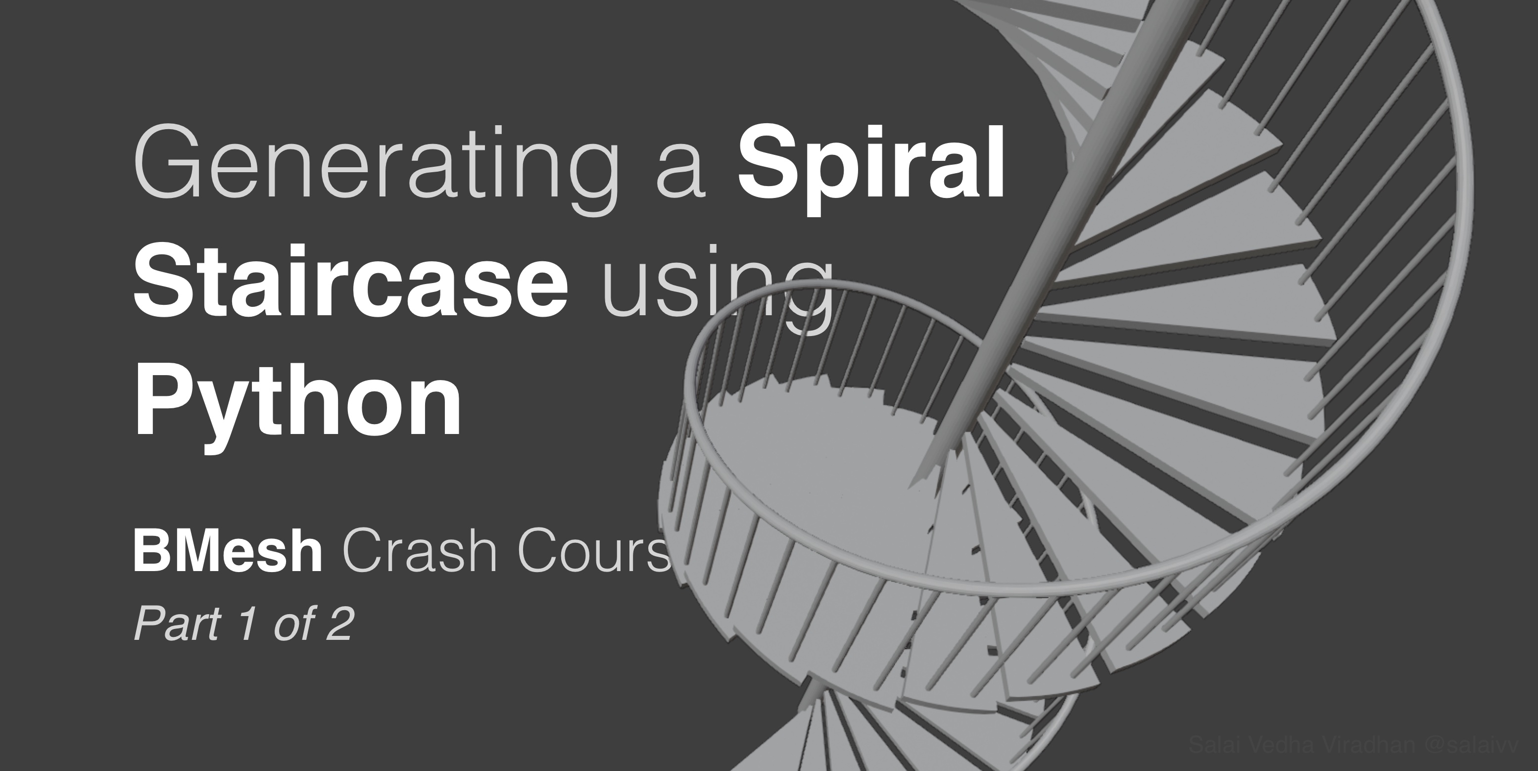
In this two part crash course, we are going to learn how to use the BMesh API by generating a spiral staircase. Here’s a summary of what we will be doing in each part:

• Part 1 – Introduction to BMesh and generating a single stair – Introduction to the BMesh API, understanding the geometry of a spiral staircase, creating a single stair using mesh operations like creating vertices, extrusion, spinning, etc.
• Part 2 – Replicating the stair and creating railing and balusters – Take the single step element from Part I and replicate it using Matrix transforms and translations to create the spiralling steps, and similarly generate the railing and balusters

Don’t be put off by the fact that we are going to be generating only a single step in this part. 🙂 We have quite a lot of ground to cover in terms of understanding the math behind a spiral staircase which will be foundational to the next part.

1. Introduction to BMesh

Although the bmesh module is standalone, we cannot directly access the meshes in our scenes from BMesh like we do using the bpy module. In fact, the BMesh module is not tied to the data present in a particular blend file at all. Every time we want to create or access mesh data from BMesh, we have to first create a new BMesh object:

import bpy
import bmesh

# Create a BMesh object
bm = bmesh.new()

Once we create a new BMesh object, we have to then instantiate the BMesh with the mesh data of an object we would like to manipulate. Suppose you want to edit the default cube, we would do something like:

bm.from_mesh(bpy.data.objects['Cube'].data)

Here the bmesh.from_mesh() method instantiates the BMesh object bm with the mesh data from our default cube. Once we do that, we can then start making changes to the mesh. For example, to change the position of a particular vertex, we would do:

bm.verts[0].co = (2, 2, 2)

Now, if you try this in the Python Console you will get an error:

Traceback (most recent call last):
  File "<blender_console>", line 1, in <module>
IndexError: BMElemSeq[index]: outdated internal index table, run ensure_lookup_table() first

This is because when we freshly instantiate a BMesh object with some data, Blender wouldn’t have the indices of the mesh elements (vertices, edges, faces) ready for us to access it like bm.verts[index]. So we need to call the ensure_lookup_table() on the element type we want to access with indices.

bm.verts.ensure_lookup_table()

In this case we are calling bm.verts.ensure_lookup_table() since we are accessing vertices by index, but the same applies to edges and faces as well. This method also has to be called every time after we create new mesh elements. Once we do that, we can then try changing the coordinate like we did above and it should run without any errors.

Now, if you notice, nothing would have changed in the viewport yet. This is because, like we discussed above, BMesh does not directly access or change data in our scenes. In order for our changes to reflect, we have to write the mesh back to the object:

bm.to_mesh(bpy.data.objects['Cube'].data)
bpy.data.objects['Cube'].data.update()
bm.free()

The update() method of the corresponding mesh is called after writing the mesh back to the object using bm.to_mesh() to ensure the updates reflect immediately in the viewport. Otherwise you have to pan, orbit or zoom once to see the changes in the viewport.

And finally we call bm.free() to cleanup the mesh data in our bm object. This method has to be called every time once we are done with our processing to free the object from memory. This step is crucial, particularly when dealing with dense meshes, otherwise we would quickly run out of memory.

So the overall BMesh workflow goes something like this:

import bpy
import bmesh

bm = bmesh.new()
bm.from_mesh(bpy.data.objects['Some Object'].data)

# Do something cool here

bm.to_mesh(bpy.data.objects['Some Object'].data)
bpy.data.objects['Some Object'].data.update()
bm.free()

There are a couple of other ways to instantiate a BMesh, but that is a topic for another day. With the introduction out of the way, let’s jump into some geometry and math.

2. Geometry of a Spiral Staircase

When it comes to the geometry of a spiral staircase, and staircases in general, there are a few thumb rules to keep in mind when deciding its dimensions.

The first and foremost being the tread and riser proportions. Tread is the horizontal plane of a step and riser is the vertical plane of step as shown in this simplified cross section:

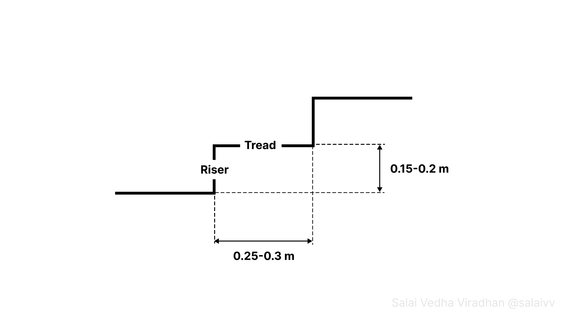
The tread depth should be somewhere between 25 to 30 centimeters for someone to comfortably place their foot and the height of a riser should be between 15 to 20 centimeters for someone to climb comfortably.

For a spiral staircase though, things get a little bit complicated because the tread depth is going to vary as we move towards or away from the center:

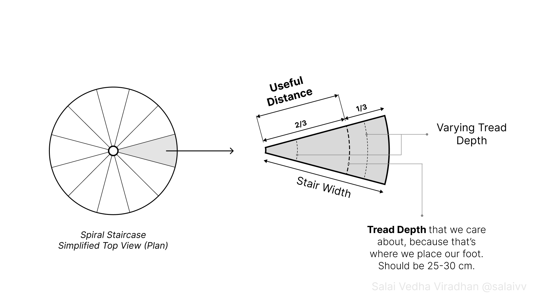
So in this case, we have something called useful distance, which is the distance from the center of a spiral staircase where someone climbing it would place their foot. It usually falls at a distance of two-thirds of the width of a stair from the center as we can see in the above diagram. We have to ensure that the tread depth at this distance (two-thirds) lies between 25 to 30 cm.

That’s not all the math we need but it good enough to conceptualise. We will have a look at the rest of the math in context along the way. 🙂

3. Generating a Single Step

Let’s start by looking at how we can generate a single step using BMesh that we can then replicate into a spiral. But before we jump into the code, let’s take a look at the following diagram (which we will look at several times during the article):

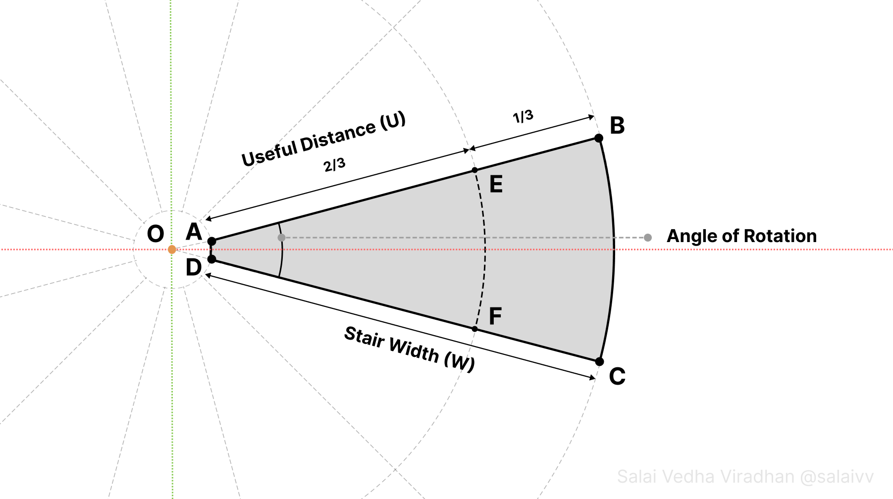
The idea is to first generate the shape ABCD along an axis, in this case the X axis, so that it is easier for us deal with rather than doing the same thing along some arbitrary axis.

If you look at the above diagram, the Angle of Rotation is the angle between the lines AB and DC, and it is also the angle at which each new step will be rotated to form the spiral. But how do we find out what this angle needs to be?

3.1 Calculating the Angle of Rotation

Well, like we saw earlier, the tread depth for a staircase has to be between 25-30 cm for a comfortable climb. And since the tread depth varies at every point along a stair, we have to ensure that the tread depth at the useful distance (two-thirds the stair width from the center) is between 25-30 cm. Looking at the diagram, we could approximate the tread depth at the useful distance as the arc length at this distance denoted as a dotted line EF.

Of course, if you were to draw a straight line joining EF, it would be slightly smaller compared to the arc length, but it is good enough approximation, especially considering the following.

If you think about it, the circumference of the circle at useful distance divided by our required tread depth would give us the number of steps we can fit inside a single circle. Dividing 360 degrees by this number of steps would then us the angle of rotation. For example, consider the radius of the circle at the useful distance for a staircase to be 0.9 m. In this case:

No. of steps = circumference at useful distance / required tread depth = (2 * Pi * 0.9) / 0.3

No. of steps = (2 * 3.14 * 0.9) / 0.3 = 5.562 / 0.3 = 18.84 steps = ~ 19 steps

Of course we cannot have floating point values for the number of steps we can fit in a circle, so we can round off the result. So we can basically fit 19 steps in a single circle (single revolution). This is not to be confused the total number steps which we will calculate later. Now dividing 360 by 19 would give us the angle of rotation:

Angle of Rotation = 360 / 19 = ~18.95 degrees

Which is, not so surprisingly, quite close to the 18.84 we got previously because the ratios between them would be the same. The rounding off explains why we got a slightly higher number this time. So we can feel confident that even if we picked 25 cm for this calculation, which is the lowest limit for tread depth, we would still be in the acceptable range even though the straight line joining EF would be smaller than the corresponding arc length.

3.2 Creating the first vertex at point A

Let’s start by creating our first vertex at point A. As we saw in the introduction, let’s start by creating a new BMesh object and setting up a few things that will allow us to iterate quickly. Open a new blend file, switch to the Scripting tab, create a new text block and copy paste the following code into the editor:

import bmesh
import bpy
import math
from mathutils import Vector, Matrix

# Parameters
STAIR_WIDTH = 1.2

bm = bmesh.new()

# We will be doing most of the work here

bm.to_mesh(bpy.data.objects['Staircase'].data)
bpy.data.objects['Staircase'].data.update()
bm.free()

There are a few things worth noting here:

• Apart from the bmesh and the bpy module, we also import the math and mathutils module. We will be using the math module to handle conversions between degrees and radians since all Blender API functions use radians under the hood.
• And we will be using the mathutils module extensively, particularly the Vector and Matrix objects for dealing with transforms like translation, rotation, etc.
• We declare our parameters at the top as constants (all uppercase letters) to which we will add more as we go. I have assumed the stair width to be 1.2 meters (or 4 feet).
• In the end, we write back the mesh to the Object Data of the Staircase object. The assumption here is that there is already an object named Staircase in the scene. Just feel free to rename the Cube to Staircase; it doesn’t matter what’s in the object as we will replace the mesh with the one we generate eventually

As we discussed earlier, even though the bmesh module is standalone, it depends on two other modules for certain things. One is the bpy module for borrowing any mesh data from the scene and to write it back. The other is the mathutils module which we will use extensively for all the math, vectors and transformations.

To create a new vertex, we use the bm.verts.new() method. It takes a Vector or simply a tuple of length 3, one for X, Y and Z coordinates, and outputs a vertex at that location. E.g.

# To create a vertex at the origin
bm.verts.new((0, 0, 0))

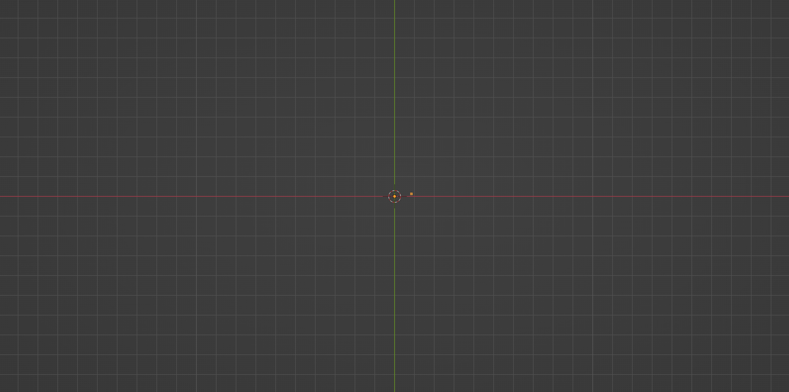
Try putting this line into our script (right after bm = bmesh.new() line; we will be following the same for the rest of the article) and try running the script by clicking on the play button on the text editor’s header. You will notice that the cube has disappeared, you will see that we have a single vertex sitting at the origin.

Now, we don’t want to create a vertex at the origin. We want our vertex at point A in our previous diagram. But how do we figure out the coordinates of this point A?

If we have a look at the above diagram, we can see that the point A lies on the line joining the origin O and the point B. The line OB makes an angle half that of the angle of rotation, because it is half of the angle between the lines OB and OC.

So putting a vertex on point A is basically the same as first putting a vertex on the X axis at a distance equal to OA and then rotating this vertex by half the angle of rotation in the Z axis with the origin as the center. But we are not going to create a vertex first and then rotate it. Instead, we are going to create a Vector object, rotate it by half the angle of rotation and then create our vertex using the resultant vector.

Let’s first create our Vector object that points in the positive X direction and has at a distance equal to OA form the origin:

...
# Parameters
STAIR_WIDTH = 1.2
POLE_RADIUS = 0.075
POLE_GAP = 0.01

...

vec_a = Vector((POLE_RADIUS + POLE_GAP, 0, 0))

...

You can see that I have added a couple of new parameter to our parameters list. The POLE_RADIUS, exactly as it sounds, is the radius of the center column or pole to which our stairs will be attached, and the POLE_GAP is a small gap between the stair and the pole. The Vector object takes a single tuple of 3 values and returns a vector object (don’t forget the extra pair of parentheses which I do quite often 😪).

We need to rotate this vector object by half the angle of rotation. So let’s start by calculating the angle of rotation first:

...

# Parameters
STAIR_WIDTH = 1.2
POLE_RADIUS = 0.075
POLE_GAP = 0.01
TREAD_DEPTH = 0.25

# Calculating Angle of Rotation
useful_circum = 2 * math.pi * (POLE_RADIUS + POLE_GAP + STAIR_WIDTH / 3 * 2)
segments = round(useful_circum / TREAD_DEPTH)
angle_rot = (2 * math.pi) / segments

...

vec_a = Vector((POLE_RADIUS + POLE_GAP, 0, 0))

...

A few things worth noting here:

• First we calculate the circumference at the useful distance useful_circum using the formula 2 * PI * radius. Here the radius at the useful distance would two thirds the STAIR_WIDTH plus the POLE_RADIUS.
• Then we divide this number by our required TREAD_DEPTH to get the number of segments. The actual tread depth would be slightly more than what we specify, which is desirable. 🙂
• Finally we calculate the angle of rotation angle_rot by dividing 2 * math.pi (360 degrees) by the number of segments we got in the previous step.

With that out of the way, we can now figure out how to rotate our vector by this angle.

To rotate vectors, the Vector object provides a built in method – Vector.rotate(other) – where the other is a Matrix representing the rotation we want to do. If you aren’t familiar with matrix transforms, I recommend checking out my one of my previous post on using Transformation Matrices and also play around with the interactive blend file to get an idea. But in a nutshell, the Matrix.Rotation() object takes three parameters:

• angle (in radians) to use for rotation,
• size (rows and columns) of the matrix
• axis (a Vector or tuple) along which to rotate

Let’s create our rotation matrix using our angle of rotation angle_rot as the angle, a size of 4 and the Z axis as the rotation axis, rotate our vector vec_a and create a new vertex:

...

vec_a = Vector((POLE_RADIUS + POLE_GAP, 0, 0))
matrix_rot = Matrix.Rotation(angle_rot / 2, 4, (0, 0, 1))
vec_a.rotate(matrix_rot)

vert_a = bm.verts.new(vec_a)
...

If you now run the script now, you will see that we a new vertex sitting just above the X axis, at a distance of POLE_RADIUS + POLE_GAP, where point A is supposed to be.

And if you notice above snippet, we are storing our vertex at point A in a variable vert_a. Because we will be be referencing this quite a few times.

But the important thing is, most of the methods, functions and operators in the bmesh module always return some useful information (some geometry or data) as opposed to operators in the bpy module where you will only receive report like {'FINISHED'} or {'CANCELLED'}. We will be leaning on this behaviour quite a lot. Now let’s create our next vertex at point B.

3.3 Extruding and creating a vertex at point B

To create our next vertex at B, we will extrude our existing vertex at A. But one thing to note about the bmesh module is that the extrude function does the equivalent of extruding a vertex with the E key and then right-clicking. This would basically extrude and create a vertex at the same location. It not provide any additional options to tell Blender where the extruded vertex needs to go. We will have to do that ourselves by moving the vertex manually after the extrusion.

This behaviour is true for most of the functions in the bmesh module – they do only one thing. This is why you would never find functions for tools like vertex slide in the bmesh module, because they are basically translations happening along an arbitrary axis, which we can achieve using transformation matrices quite easily.

With that in mind, let’s extrude our vert_a first to create a new vertex which we will eventually move to point B:

...

return_geo = bmesh.ops.extrude_vert_indiv(bm, verts=[vert_a])

...

We extrude vertices using the extrude_vert_indiv() method in the bmesh.ops sub-module. This method takes two inputs, a bmesh object and a list of vertices, and extrudes them and puts them in the same place. In our case we pass the bm variable that holds our bmesh object and a single vertex vert_a inside a list and we store the result in a variable named return_geo.

If you try printing return_geo, you would see something like this:

{'edges': [<BMEdge(0x2980a0010), index=0, verts=(0x125853010/0, 0x125853048/1)>], 'verts': [<BMVert(0x125853048), index=1>]}

The extrude method has returned a dict object containing two list – one containing edges and the other containing the vertices created as a result of the extrusion. In this case, in the verts list we have a single vertex which we will be moving to point B. Let’s store this vertex in a variable named vert_b:

...

return_geo = bmesh.ops.extrude_vert_indiv(bm, verts=[vert_a])
vert_b = return_geo['verts'][0]
del return_geo

...

I have also gone ahead and deleted the return_geo variable since we don’t need the rest of the data and also because we will be using the same variable name for subsequent bmesh operations, so that we don’t accidentally access the old/incorrect data.

Now let’s figure out how to move this vertex to point B. Let’s have another look at the same old diagram again:

The line joining OB would make the same angle with X axis as the line joining OA would. So we don’t have to go through the same process of creating a vertex on the X axis at some distance (stair width) and then rotating it about the origin by that angle. Instead, this time let’s use the point A as a reference for the transformation.

In vectors, there is a concept of scaling, which is nothing but multiplying a vector by a number. This would basically move the end point of a vector towards or away from the origin depending of if the number by which you multiply is less than or greater than 1 respectively.

In this case, the vector OB is a scaled version of the vector OA by some factor. To find out this factor, we can simple divide the length of OB by OA:

scale_factor = (vec_a.magnitude + STAIR_WIDTH) / vec_a.magnitude

Here we are dividing the sum of magnitude of vector OA and the stair width, which is essentially the length of the vector OB, by the magnitude of vector OA. Now multiplying the vector OA by this scaling factor would gives us the vector (or coordinates) of point B, Which we can assign as the coordinates to our vertex stored in vert_b:

vec_b = vec_a * scaling_factor
vert_b.co = vec_b

At this point, this portion of the code should look something like this:

...

return_geo = bmesh.ops.extrude_vert_indiv(bm, verts=[vert_a])
vert_b = return_geo['verts'][0]
del return_geo

scale_factor = (vec_a.magnitude + STAIR_WIDTH) / vec_a.magnitude
vec_b = vec_a * scaling_factor
vert_b.co = vec_b

...

If you run the script now, you will notice that we have a single edge, denoting AB, in our viewport:

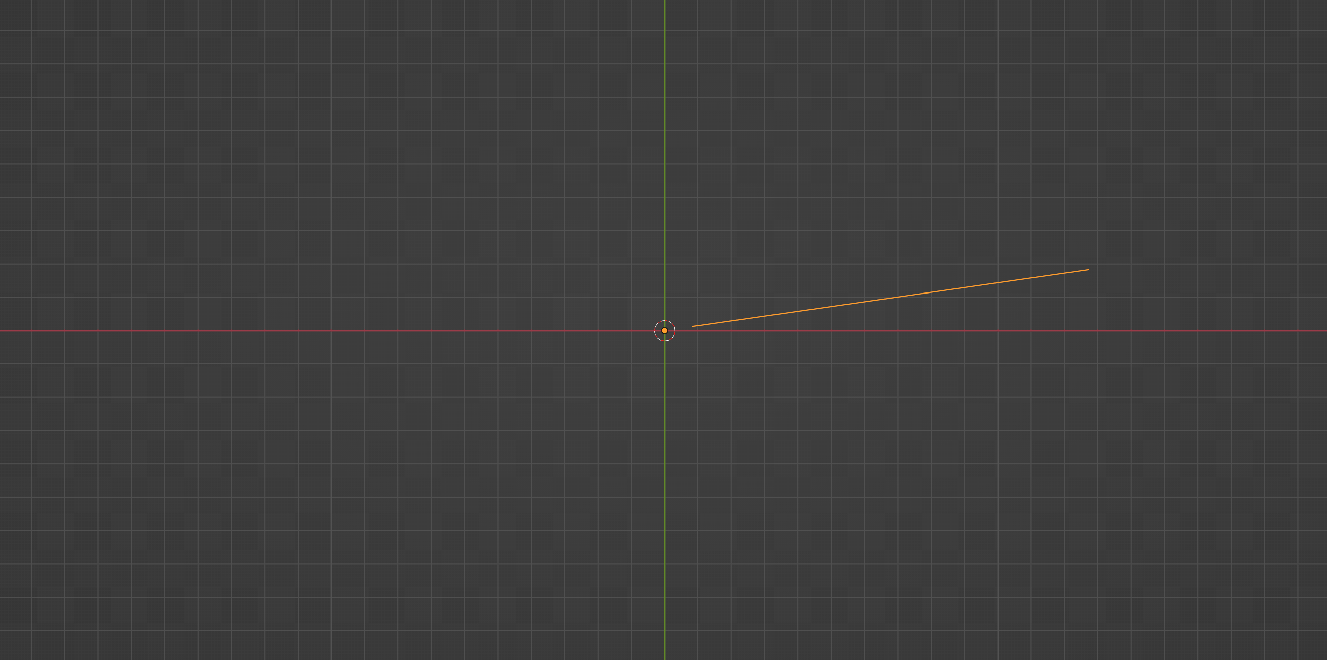
Now let’s have a look at generating the arc connecting point B and point C.

3.4 Creating the arc connecting B and C

So far we have looked at how we can use vectors and matrices to mathematically derive the coordinates we need and to create or place vertices at these locations. For the point C, we are gonna directly use a method from the bmesh library without having to calculate C’s position – the bmesh.ops.spin() method.

Most of us would have used the Spin tool when creating 3D models. This is the underlying bmesh operation that the Spin tool uses, and it takes several parameters:

• bm – the bmesh object, as usual (all bmesh operation expect this)
• geom – a list of mesh elements for which we will be providing a single vertex vert_b
• angle – the total angle of rotation for the spin; the angle_rot in our case
• steps – how many vertices to use for the spin; higher the number smoother
• cent – the center (Vector or tuple) about which to perform the spin; the origin in our case
• axis – the axis (Vector or tuple) in which to perform the spin; the Z axis in our case

Let’s give it a try. In my case I have decided to use a step count of 8, but feel free to play around with the numbers:

...

return_geo = bmesh.ops.spin(
    bm,
    geom=[vert_b],
    angle=-angle_rot,
    steps=8,
    cent=(0, 0, 0),
    axis=(0, 0, 1)
)

...

If you notice, I have prefixed a - sign in front of angle_rot, because by default the spin happens anti-clockwise. And for the center and axis, I have use (0, 0, 0) and (0, 0, 1) to denote the origin and the Z axis respectively.

If you run the script now, you should be seeing something like this in the viewport:

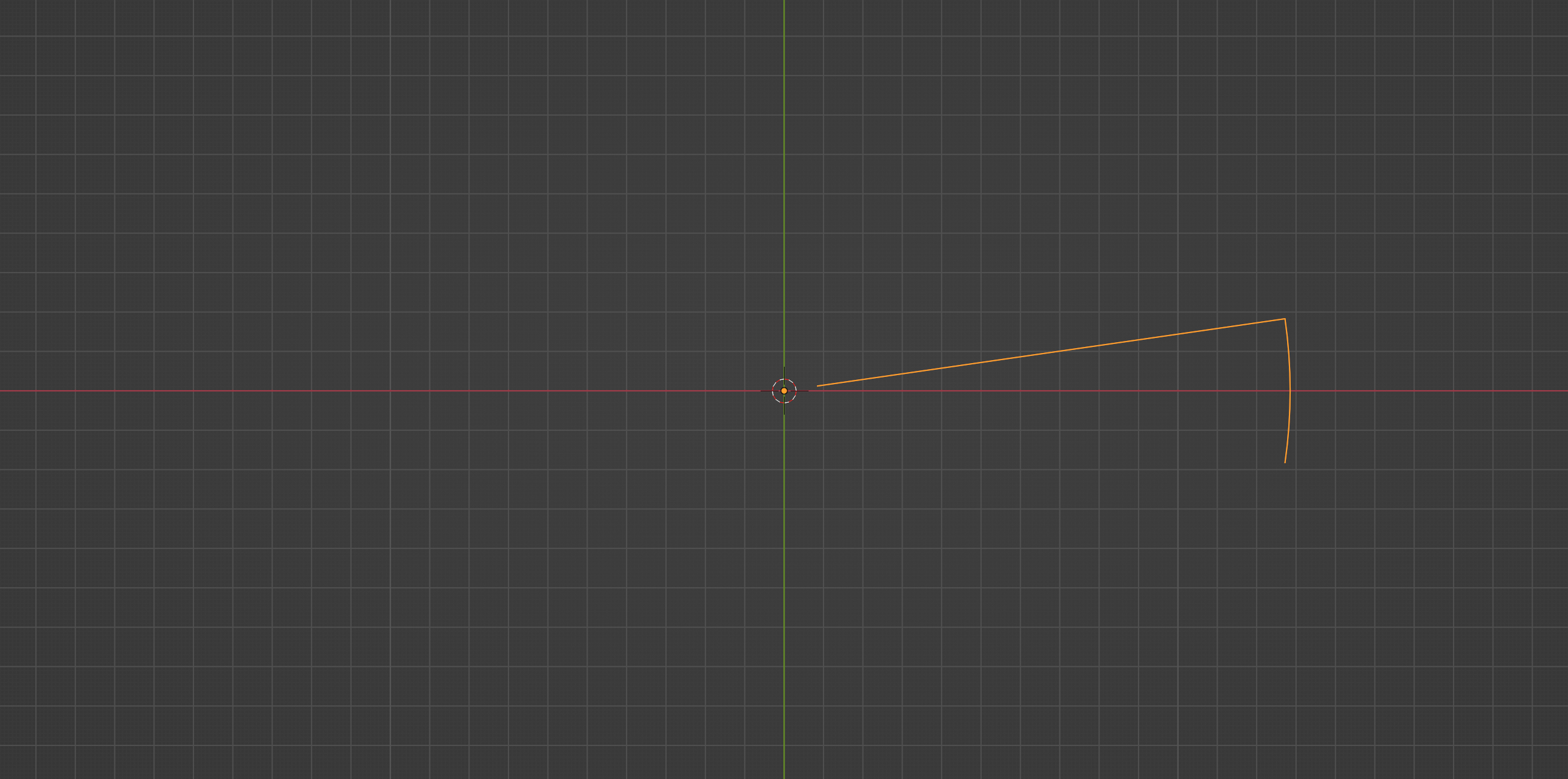
If you print the return_geo variable, you can see that it has returned the last vertex of the spin operation:

{'geom_last': [<BMVert(0x12d038608), index=9>]}

Which is basically our vertex at point C. Let’s store this vertex in vert_c and delete the return_geo as usual:

...

return_geo = bmesh.ops.spin(
    bm,
    geom=[vert_b],
    angle=-angle_rot,
    steps=8,
    cent=(0, 0, 0),
    axis=(0, 0, 1)
)

vert_c = return_geo['geom_last'][0]
del return_geo

...

Now let’s move on to generating the last vertex at D. A little more vector math. 🙂

3.5 Creating the last vertex at point D

To create our vertex at D, we are going to use the extrude method again, but before that we have to find out the coordinates of D. Once again, last time I promise, let’s have a look at our diagram:

From the diagram, it’s apparent that the coordinates of D are going to be same as A but with their Y coordinates flipped. So all we need to do is extrude to make a copy of vert_a’s coordinates and flip the Y axis coordinate:

vec_d = vert_a.co.copy()
vec_d.y *= -1

Let’s now extrude and move the resulting vertex to this location:

return_geo = bmesh.ops.extrude_vert_indiv(bm, verts=[vert_c])
vert_d = return_geo['verts'][0]
del return_geo

vert_d.co = vec_d

With that we now have all the vertices required for a single step. All we have left to do, if to create a face with the vertices we have and extrude them to give it some thickness.

3.6 Creating a face and adding thickness

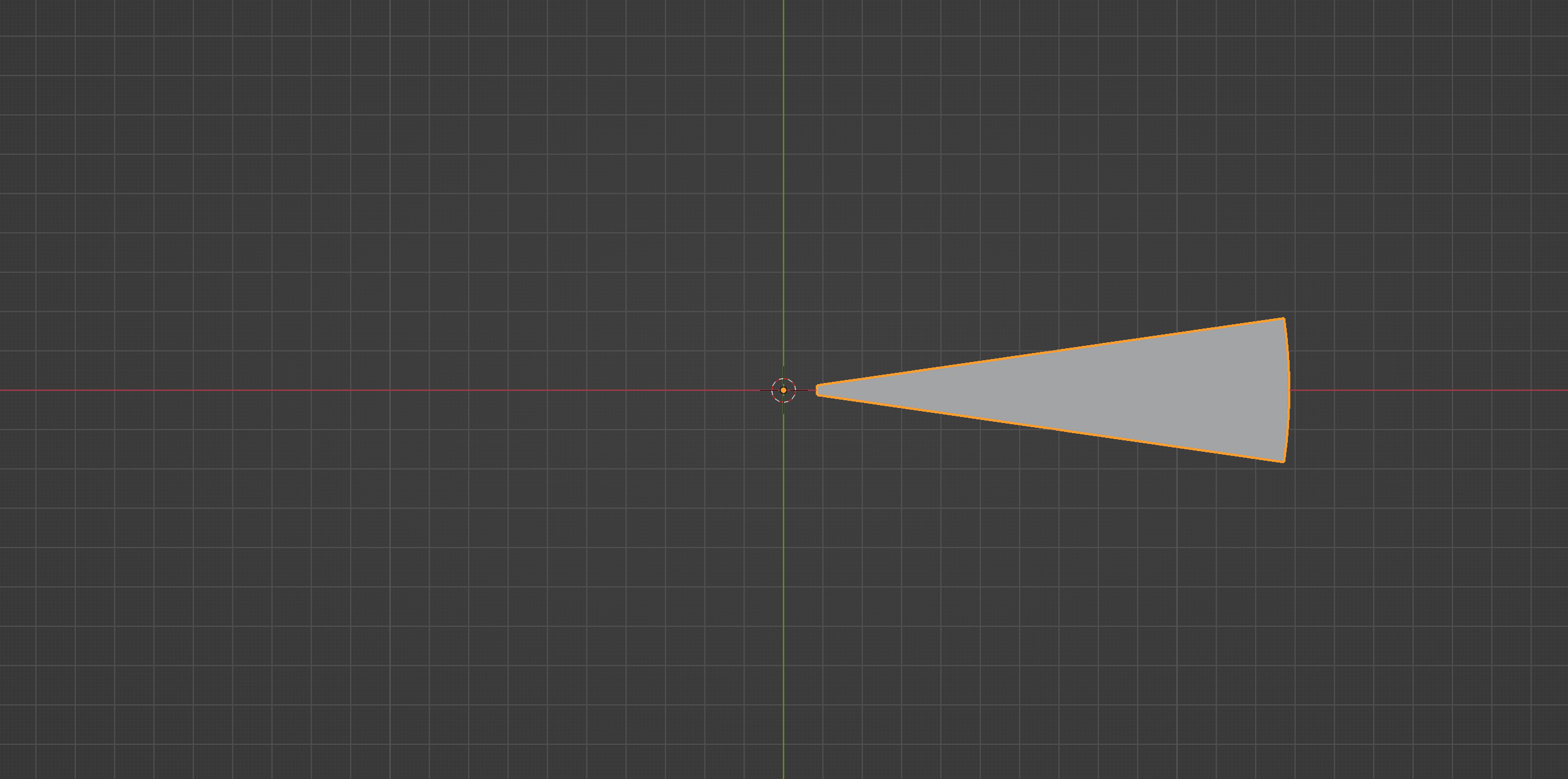
To create new mesh elements, like edges or faces from existing vertices, we can simply use the new() method on the respective element type and provide it with the required geometry. In our case, to create a face, we have to use the bm.faces.new() method and provide it with the vertices that will make up with face:

stair_profile = bm.faces.new(bm.verts)

That’s all it takes to create a new face. Notice that we have provided all the vertices in the mesh by passing bm.verts since we only have those vertices. But you could provide a subset as well. If everything went well, upon running the script, you should see something like this:

In order to add thickness to the the stair, we can use the same extrude and move technique, but this time with the face as the input:

return_geo = bmesh.ops.extrude_face_region(bm, geom=[stair_profile])

Now, in bmesh, there is no concept of moving a face. Instead we have to move all the vertices that make up that face in the direction we want. In our case, we first need all the vertices that make up the newly extruded face. And as always, we can get this information from our return_geo from the extrude operation.

But the return_geo contains all the resulting geometry in a single list under the 'geom' key, so we have to extract the vertices from this list:

verts = [elem for elem in return_geo['geom'] if type(elem) == bmesh.types.BMVert]
bmesh.ops.translate(bm, verts=verts, vec=(0, 0, -TREAD_THICKNESS))

You can see that we loop through every element in the list, and check if it is a vertex by comparing type(elem) with bmesh.types.BMVert, which is the internal type for a vertex. We then translate these vertices using bpy.ops.translate() by providing this list of vertices.

Notice I have used the negative value of TREAD_THICKNESS as the Z coordinate to extrude the stair profile downwards. Add this at the top to our parameters list; I used a value of 0.05 for the thickness.

And that’s it. If you have got everything right so far, upon running the script you should see something like this in your viewport:

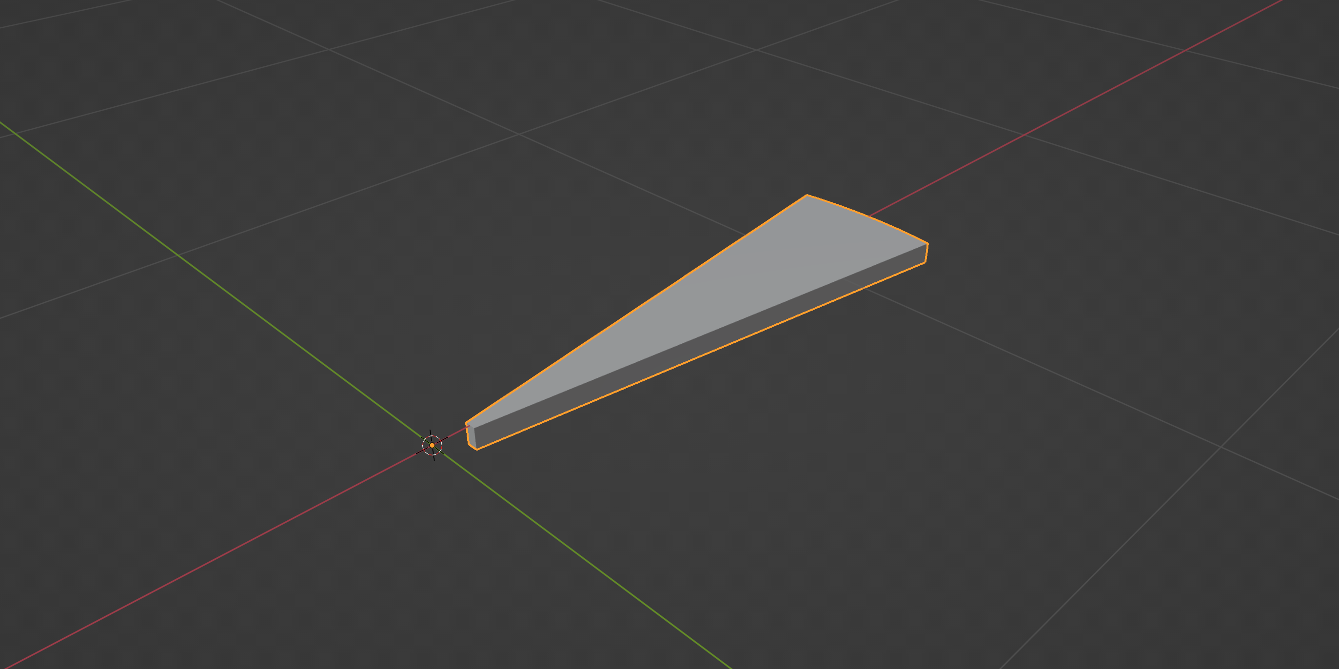
Play around with the parameter values and see how it affects the shape of our stair element. Kudos if you have made it this far!

One interesting thing to note is that we never called the ensure_lookup_table() method, that we saw in the introduction, even once during this process. Because we never had the need to access vertices, edges or faces using indices directly from the bm object.

Since bmesh operations return some useful information, we can do subsequent operations using this data without having to deal with the entire bmesh object. So use this method only when you need to.

Conclusion

In the next part, we will be looking at generating the staircase by replicating this stair element, and also create the rest of the parts like the pole, railing and the balusters. You can grab the finished blend file from this link.

Make sure you are subscribed to receive the next part directly to your inbox. Stay tuned! 🙌🏻

Read the Part 2 article here.

Resources

• BMesh API documentation
• mathutils documentation
• Linear Algebra series by 3Blue1Brown